
Unit tests are indispensable for reliable, robust code. They give confidence that the code works now, and that any needed changes can be made safely in the future. Well-written tests also serve as documentation for the actual behavior of the code, as opposed to separate documentation which often falls out of date.
All of these benefits hold true for code within Jupyter Notebooks. However, as the notebooks themselves are not pure code (the .ipynb files are JSON), they cannot be easily imported into external test files. There are a few different ways to get around this:
- Avoid importing by including test assertions in-line. This is the easiest method, and it technically works, but it clutters the production notebook with tests cases and it’s not fully automated.
- Move code into external files (.py), and then import these into both the Jupyter Notebook and the test files. This probably feels the most natural to a software engineer, but it goes against the grain of Jupyter Notebooks by separating the notebook’s code from the inline text and data output. It also complicates the execution of the notebook itself, especially in cloud environments.
- Add a module that allows Jupyter Notebooks to be imported. This preserves the benefits of Jupyter without cluttering or modifying the original notebook in any way.
We will demonstrate this third approach, using ipynb to import our notebook into additional testing notebooks. Then we’ll collect and run these tests using pytest with the plugin nbmake.
A key benefit of this approach is that we can develop our tests just like we do our main notebooks. We can experiment with test code and visualize the results as we go, which works surprisingly well for approaches like test-driven development (TDD).
Demo Background: Battery Charging Statistics
For our demo, imagine you use the Losant Platform to manage a fleet of asset tracking devices with a built-in battery. You know that for these devices, battery life is prolonged if the battery isn’t recharged until it is at least 80% discharged. But what’s happening in the real world? When are users actually charging the devices?
To answer this question, you decide to make a notebook to create a 30-day summary report on battery recharging behavior. The notebook will use the devices’ state history to identify when users began charging devices, and will then output a summary of these rows into a data table.
Application Setup
If you haven't already, sign up for a Losant sandbox account and create an application using the template, “Asset Tracking”.
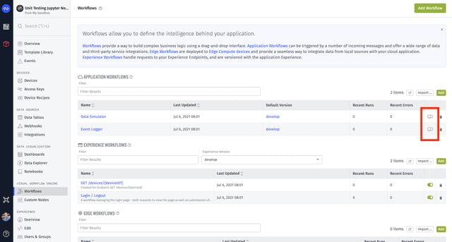
When the application is created, visit the Workflows page and toggle the “Data Simulator” workflow on. This will begin simulating data every two minutes for the five asset tracker devices the template comes with. If you like, go to Dashboards and visit the ”Overview Dashboard” to view this data as it comes in.
While the data is being simulated, let’s set up our Notebook. Go to Notebooks and click the green “Add Notebook” button. Name the Notebook “Battery Statistics,” leave the Image Version field alone, and hit “Create Notebook”
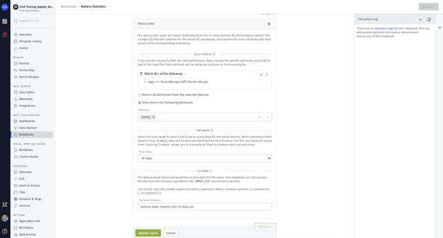
Now we need to give the Notebook some input data. Click “Add Input-> Device Data”.
- Under “Select Devices”, click the Edit icon to change the filters to “Match ALL of the following… tags === DeviceRecipe = GPS Tracker Recipe”.
- Choose “Only return the following attributes: battery”.
- Leave the time range set to “30 days”.
- Set the “File Name Template” to “battery-state-reports-last-30-days.csv.”
- Click “Update Inputs”.
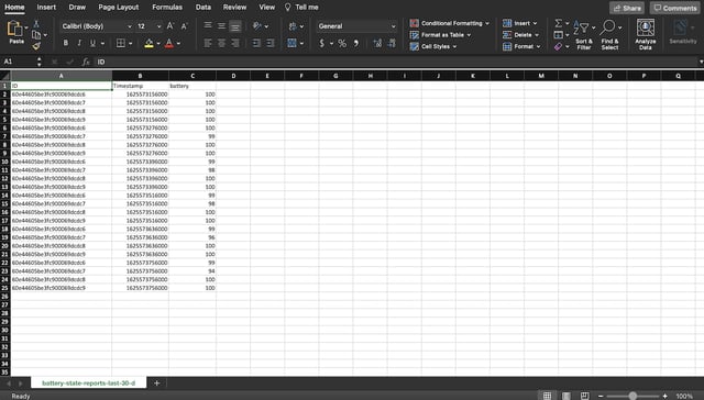
 Once you have enabled the data simulator you will need to give this step some time. Then, under the data input field on the same page, click the “Request Data Export” button. This will send a sample export to your email address.
Download the file when it arrives, and you’re ready to begin creating the notebook.
Notebook Setup
With Losant, you develop your notebooks locally and then upload them for execution on the cloud.
Install the needed python packages. This tutorial assumes you already have python and JupyterLab installed on your computer. If not, install python and then JupyterLab. You’ll also need the following dependencies:
- ipynb (pip install ipynb)
- nbmake (pip install nbmake)
- pandas (pip install pandas)
Create a local directory for your project, and place the “battery-state-reports-last-30-days.csv” file you downloaded from the data export email there.
From a terminal, run JupyterLab from that directory, and it will open Jupyter in a new browser tab.
Click the “Python 3” icon to create a new Jupyter Notebook. Rename it to “battery-stats.ipynb” in the sidebar.
Paste in this starting code to load the input file into a DataFrame. It pulls directly from the Losant input files if executing on the cloud, or from the current directory if executing locally (as we are doing now).
To gather insights into when users are charging their batteries, we need to isolate the rows immediately before the user begins charging the device. We’ll create a function, “get_rows_before_charging”.
Of course as this is written it just returns the DataFrame back out unchanged. Let’s write this function using TDD.
Writing Tests
In the side-panel, click the “+” button and create a second notebook. Rename it to “test_get_rows_before_charging.ipynb”.
We can use the “ipynb” module we loaded earlier to import the first notebook:
A great thing about the ipynb module is the option to only import the definitions (and globals) using the “ipynb.fs.defs” syntax. So it won’t actually execute any code when we import it like this.
Now that we have a reference to our function, we can write our first test:
What should our test data look like (“???” in the snippet above)? Well, we want it to match the real data as closely as possible. This is where developing tests in a notebook shines! Let’s create some quick cells to examine the data. Borrowing a few lines from the first notebook, we can take a look at the structure of the data using df.dtypes and df.head().
Now we can create mock data using this information. To create many test cases, doing this with a function is helpful:
Note we are being careful about dtypes — otherwise pandas will try to determine the most appropriate type based on the values, and we do not want that variance.
The cells we created to look at the real data can now be deleted, and then we can use our function to easily create mock data for our first test:
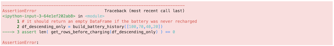
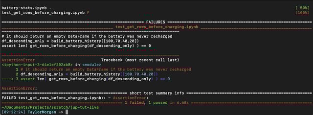
Running the notebook within Jupyter, we can see if our assertions pass or fail. In this case, it fails because we haven’t implemented any logic at all.
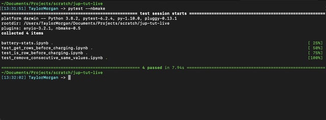
We’ll fix that in a moment. First, since we eventually will have multiple tests in multiple files, we want to be able to run them on the command line. In the same directory:
pytest –nbmake
We should see it gather and run the first test. Note that while nbmake allows pytest to pull and run notebook files, it will not automatically execute test functions. With test notebooks, we just leave the assertions in the outer scope.
It’s time to make our function pass this first test:
Re-run the test, and it passes! (Caution: You may have to restart the kernel of the test notebook (Kernel -> Restart) when function definitions and input files change.)
If it hadn’t, we could output the actual results right in the test notebook. It’s super helpful in writing our tests to not have to print a bunch of debug statements, plus the output can be much more user-friendly using all that Jupyter has to offer.
Completing the Remaining Tests
Of course, this function is quite inaccurate. It’s simply returning rows where the next row has a higher battery reading, i.e. the device is charging. It won’t isolate the rows where that starts happening, and it won’t handle non-changing rows well either (e.g. 70->70->80). We continue through the TDD process: writing tests, adjusting our function to pass, and refactoring.
Skipping ahead through this iterative process, we end up with several more test cases for this function, as well as two helper functions which also get their own tests.
Inside battery-stats.ipynb:
test_get_rows_before_charging.ipynb:
test_is_row_before_charging.ipynb:
test_remove_consecutive_same_values.ipynb:
Executing and Saving Results on the Cloud
With confidence that this function is accurately returning only those rows immediately before a charging event, it’s trivial to get summary data about them: get_rows_before_charging(df)['battery'].describe() gets us most of the way there, returning the mean, min, max, std, and several percentile values as a Series.
Our export function can transpose this into a DataFrame with data table friendly names before saving it as a csv:
The complete source can be found at Jupyter Unit Testing Demo.
We can upload the notebook directly to Losant, and it will automatically bundle the device data as an input, execute the notebook on the cloud, and save any output.
First return to the Losant application, go to Data Tables, and create a new one. Call this “battery charging stats” and save it without any columns.
Then return to the notebook page from which we exported the sample data. On the “Notebook File” tab, upload the "battery-state.ipynb" notebook file.
Note: Losant does not curently support the 'id' property in Jupyter 3 cells. Check in the notebook source that these have not been added automatically if you have trouble uploading. You can safely delete them.
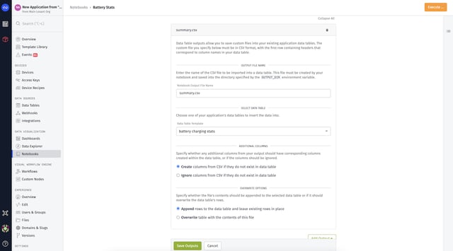
Finally, configure the output so that it processes the summary csv file we exported and saves it in our table. On the “Outputs” tab, click the “Add Output->Data Table” button. The output name should be “summary.csv”, the table is “battery charging stats”, it should append rows, and it should create columns as needed.
Now you can execute the notebook directly using the button at the top of the notebook page.
Note: Depending on how quickly you followed this tutorial, the simulated devices may not have had any recharge cycles yet. It’s best executed after a day or so, but you can try and see your results; one of the output columns is the count of matching rows.
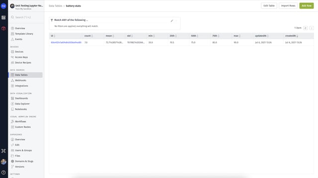
After the notebook finishes executing, check the results in the Data Table.
Going Forward
Rather than execute the notebook manually, we can easily set up a workflow to execute it on a timer. A simple application workflow might look like this:
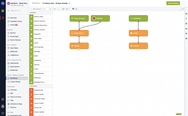
The left path is triggered by a timer every 30 days, kicking off the notebook’s execution.
After the notebook execution completes, the Data Table will be updated with the latest summary data. The right path in our workflow is just for convenience. It is triggered when the notebook execution completes, sending us a summary email with a link to the output file.
For future development, we save the test notebooks, and run the suite every time we need to work on the notebook. For instance, if the manufacturer later tells us the battery sensor has a +/- 2% accuracy, we can go back, add some test cases to account for this, and then update our notebook’s logic to only pull rows before a cumulative 3% rise.
Summary
We've created an automated test suite for a Jupyter Notebook, without cluttering up the notebook or relying on manual test running. We can now develop confidently, refactor, and have confidence that our notebook is processing data correctly. Our solution is highly extensible, as we can create as many test files as we need. Finally, since we develop our tests directly inside of another Jupyter Notebook, we get all the benefits of running and visualizing our code outputs as we develop.
Our team is standing by to answer any questions you have. Please contact us to learn how Losant can help your organization deliver compelling IoT services for your customers.