
In part 1 of this 2-part series, we looked at a few ways to use software to filter out noisy sensor data. Our case study is a municipality monitoring the depth of a storm water system, using two separate sensors with different strengths and weaknesses.
With some simple techniques, we were able to accomplish quite a lot. First, if our visualization is our only goal, then the Time Series Block’s aggregation methods already gives us everything we need to smooth out our data’s representation. Second, using a workflow to calculate a combined average brought our sensor readings together, and using a running average allowed us to dampen the effect of outlying sensor data. Finally, deriving a pattern—the rate of change—and building it into our estimate using linear regression allowed us to loosely predict the next readings and prevent our estimate from lagging behind changes.
The Kalman Filter will allow us to do all of these things as well, but with a more robust probabilistic framework. Our end result will be Losant Dashboard very similar to the one we arrived at in part 1:
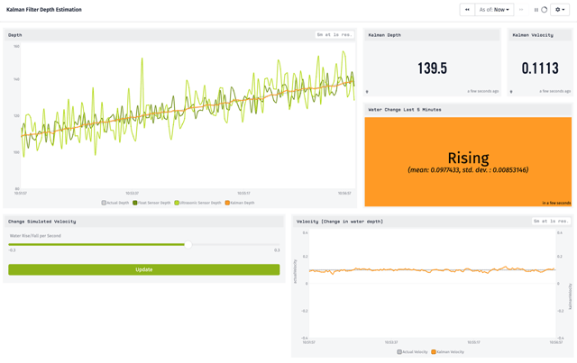
The main chart in the top left graphs each sensor’s noisy reading (light and dark green) as well as our estimate derived with Kalman Filtering (orange). On the right we have our current estimate of the water’s depth and the rate of change, as well as a chart and indicator showing our statistical belief in that rate of change (shown here as “Rising” at a rate of .067 cm/s, with a standard deviation of 0.013 cm/s). The controls are used only for the simulation, changing the actual water level and resetting the Kalman Filter.
Kalman Filter
In short, a Kalman Filter works by maintaining an estimate of state and predicting how it will change, then comparing that estimate with observed values. Both the expected and the observed values have an amount of uncertainty associated with them. The algorithm adjusts its belief for the next cycle by resolving the difference between the expected and observed values according to these uncertainties.
That’s a bit of a mouthful, but it will become a little more intuitive with our concrete example. If you’d like a more thorough explanation of Kalman Filters, I recommend Brian Douglas’ introduction which offers an excellent balance between thoroughness and simplicity.
In our storm drain water level example, we will maintain a belief about the current water depth and the depths’ rate of change (velocity). Combined, these are our state, which is just our best guess. We will also maintain estimates of how confident we are in these values, expressed with variances. Together these variances are known as the P matrix.
If you’re familiar with probability, you may notice that at this point we essentially have gaussian distributions. By definition, a gaussian distribution is one that can be presented by a mean and standard deviation. You can see these drawn in on the axes of this chart:
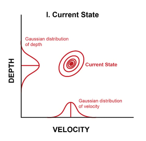
We use a matrix for tracking the variances so that we can estimate covariances as well. Covariances are a measure of how variables affect each other. For instance, the more we think the depth’s rate of change is, the higher we will expect its depth to be. This gives the gaussian its diagonal appearance in the chart above. At this point we have accounted only for the uncertainty in our existing estimate.
Next, we will create a linear model of how this state changes from one step in time to the next. For depth, this will simply be that the next depth = the last depth + the rate of change. We will not expect the velocity to change of its own accord (we are not tracking any type of acceleration). This transformation recipe is known as the F matrix. So here already is one place where we are building in our knowledge of the system, i.e. that there is a reasonable expectation for a somewhat consistent rate of change.
If we knew of other external factors (say, a valve opening that would increase the flow) we could apply those transformations at the end of this step, which is known as a U matrix. For simplicity, we are not using a U matrix here.
Applying the F matrix to our current state, we create a prediction:
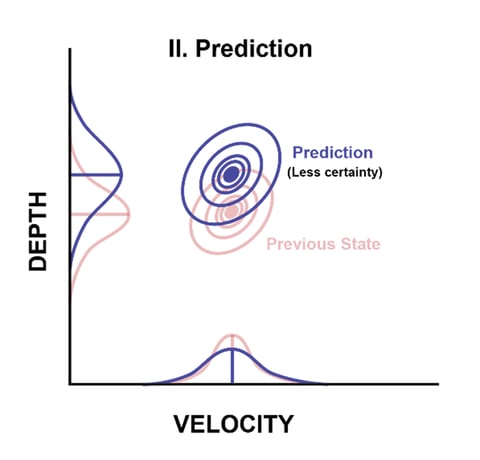
Remember, we are only using our current state and our knowledge about how it behaves here. Notice that the variances grew larger. We are estimating into the future, so we are less confident about the values. In fact, we can choose to add in additional hard-coded variation known as process noise, or the Q matrix, to represent our uncertainty in our model.
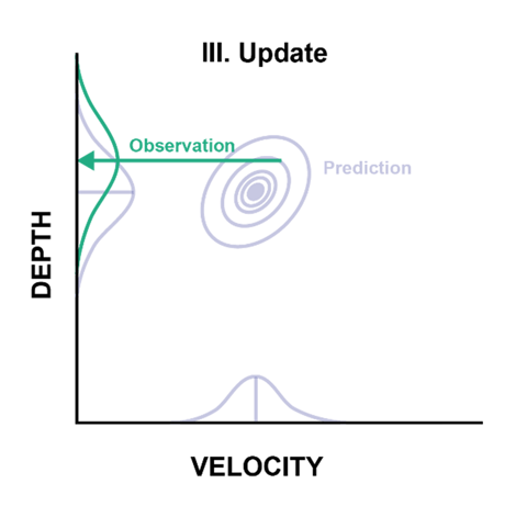
This prediction step was the first of two key Kalman phases. The second is when we update our prediction based on new observations—specifically our sensor readings. Due to sensor noise that we write into our Kalman Filter (more on this below), these observations also have their own gaussians:
Deciding how much variance to assign our observations is part of refining our Kalman model. In this case, we have some information about their accuracy, so we can start with those values. We’ll likely adjust them as we fine tune our model to account for other factors like water churn. In any case, the observation uncertainties are known as the R matrix, and the resulting probability distribution is shown visually along as the axis.
The example chart above shows the sensor reading came in a little higher than we expected, which also means that the velocity was a little higher than expected (only one sensor’s gaussian is shown on this chart). With this reading, we are ready for the update phase of the Kalman Filter process.
We combine our prediction and observation, weighting the result by how much deviation each distribution has:
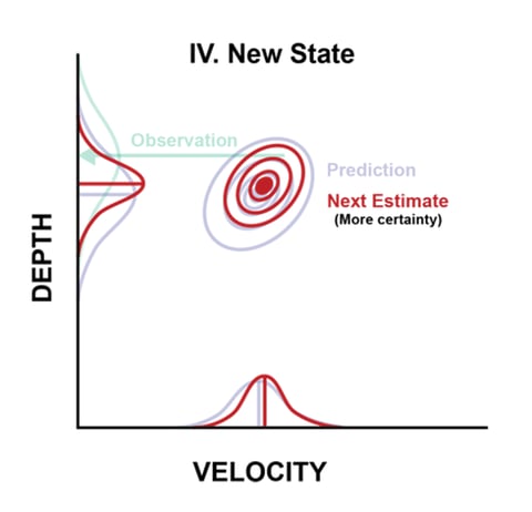
We end up with an updated and more accurate estimate, and the process starts over. Thus we have a cycle of predictions and observations. When we predict, we lose a little bit of certainty. When we get new data, we gain a little bit of certainty. The exact specifics are largely handled by the Kalman Filter formulas, which use a lot of linear algebra to deal with all the matrices. Other than implementing these, most of our work is fine tuning the different variables that controls how the filter behaves (for instance, how much noise each sensor has).
Finally, in our example, we have two sensors giving readings. We essentially perform Predict -> Update -> Update. More sensor data can only help us.
Implementing the Kalman Filter in Losant
In part 1, we discussed using 2 separate attributes on a single device to track the sensor readings. Here we’ll add a third depth attribute to track our best estimate using the Kalman Filter. We want to make sure to keep these 3 depth measurements (2 sensors + 1 estimate) separate. We don’t technically have to store the observations for Kalman to work, but we want to see them on the graph.
In addition to the depth, we’ll also set up attributes for the estimated rate of change (velocity) and the P matrix. As a reminder, the P matrix holds the variances and covariances of our current estimate. Even though we’ll only ever use its last value, storing it as Device State makes more sense due to how frequently it will be changing.
We want the Kalman Filter to run every time we receive new telemetry, since the new observations will improve our depth estimate. Just like we did in part 1, we’ll set up a workflow that’s triggered by our device receiving its sensor data. This time it will run the Kalman process, and then update the device’s state with the new estimates.
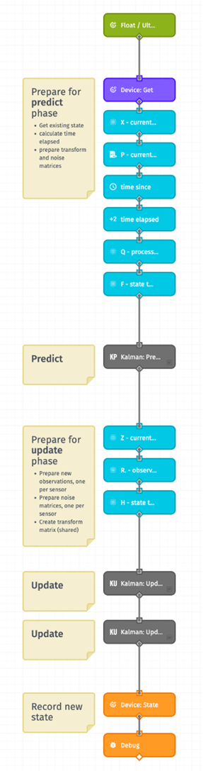 |
The workflow is triggered by the device receiving new state for the floatDepth and/or ultrasonicDepth. We’ll prepare the latest depth estimate (X), velocity estimate and covariance matrix (P) using the values from the composite state of the Device: Get node. Since we use the velocity to estimate how much the level has changed over time, we also need to calculate how much time has elapsed. Finally, we set up the transformation matrix (F) and a little bit of hard coded noise (Q) to account for our reduced confidence in future estimates. Now we run the Kalman Prediction, using a custom node (explained in more depth below). Next we prepare for the update phase by readying our observations (Z) from the state report that triggered this workflow. We also set up the observation noise (R) matrices—one per sensor—and a simple utility matrix (H) that converts between our tracked Kalman state (two values, depth and acceleration) and our observations (a single value, depth). We run the Kalman Update phase once per new observation, again using custom nodes. The first takes in the result of our predict phase, and the second takes in the result of the first update. In other words, they are processed serially. Finally, we save the new depth, velocity, and P matrix as device state. |
|---|
Encapsulating the Kalman phases in custom nodes makes it very simple to control the overall logic flow. For instance, it was trivial to add a second observation step. By setting up all of our matrices in this outer workflow, it’s also simple to fine-tune the actual values without the mess of the Kalman formulas. Then we simply pass these matrices to the custom nodes.
Tuning our Filter
We have to tune our filter values to approximate our belief of the sensor noise and environmental variations. First, we express our belief of how much our estimation process loses accuracy, the so-called process noise. After some experimentation, we’ll settle with a process noise (Q) matrix of:
[0.003 0]
[0 0.00005]
The top left value here is additional variance for the depth, and the bottom right is additional variance for the rate of change. Remember we are storying two variables in state (depth and velocity) so we have 2x2 matrix. Here .003 is added to the variance of the estimate of the depth, and .00005 is added the variance of the velocity. No amounts are added to the covariances. Higher values (say, 1 and .01) resulted in much more erratic values. Lower values (even 0 and 0) created smoother, more stable values, but ones that did not catch on to real changes very quickly. It can be quite a bit of trial and error to get stable values that also respond to real changes.
In part 1, we did not take the sensors’ accuracies into consideration, other than to try to eliminate the resulting noise. The Kalman Filter, though, naturally incorporates observation uncertainty in the form of the R matrix. This is the gaussian distribution seen in green on the charts above.
For the float sensor noise, we find a value for the observation uncertainty matrix that works well of [25]. This is a 1x1 matrix because there is only one value with the sensor readings. This number may seem high, but it has to account for both the sensor’s inaccuracy (+/-4 cm) and the natural churn of the water. Variance is also the standard deviation squared (which would be 16 just for the inaccuracy of the sensor), so 25 is not significantly higher.
If the value we choose is too high, the depth estimate will be more stable but will also be slow to respond to true depth changes. If it’s too low, the estimate will start to exhibit the erratic behavior of the sensor readings as it pays too much attention to each reading.
The ultrasonic sensor’s R matrix is similar to the float sensor’s, but has a variance that is affected by the distance of the sensor to the water level. If the sensor is mounted at 10m high (=1,000 cm), the distance is 1,000 minus the previous estimated depth of the water. (To make sure our distance stays above 0, we’ll set a maximum height for this calculation of 999cm.) In the end, we’ll use:
| 1000-min(depth,999) 10 |
+ 5 |
|---|
With this equation, a high water level of 900cm yields a variance of [15]. A low water level of 50cm yields a variance of [103.5].
Inside the Kalman Filter Algorithm
Let’s take a look under the hood of the Kalman: Predict custom node.
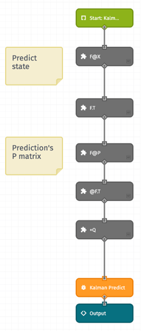 |
The formulas for the prediction result in estimated values for state (X) and the covariance matrix (P). They are often written with a ˆ, or hat. X_HAT = F @ X Since the F matrix transforms the current state to the next state, it is a simple matter of taking the dot product (@) of those two matrices. We’re using 3 custom nodes for the matrix operations here: Matrix Transpose, Matrix Multiply, and Matrix Arithmetic. We will do the same for the updated P matrix, with the result multiplied by the transposed transformation matrix and the process noise added in. |
|---|
The Kalman: Update custom node works very similarly, albeit with more steps:
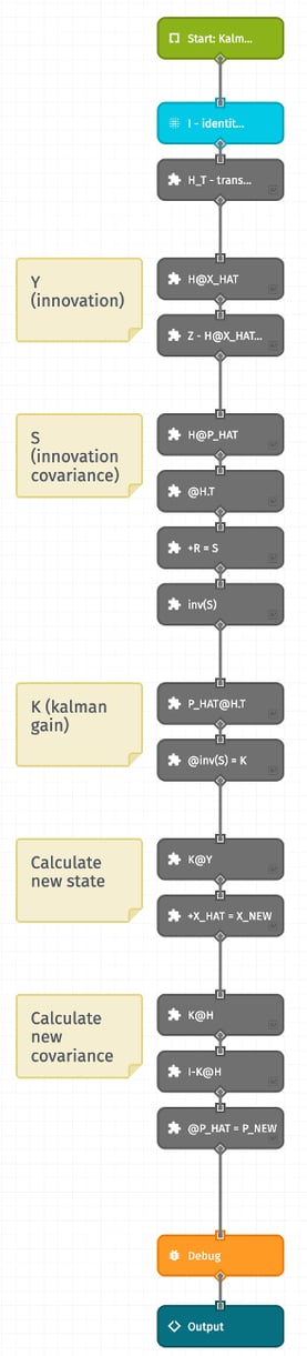 |
The formulas for both prediction and update phases give updated values for the state (X) and the covariance matrix (P). To distinguish these from the predict phase, we will refer to them here as X_NEW and P_NEW. The update step formulas are: Y = Z-H@X_HAT We first calculate Y, the innovation, which represents the difference between our predicted value and the observed value. Next, we need S, the innovation covariance. This is the sum of the estimate’s covariance and the observations covariance. They have to be adjusted to be in the same dimensions first. Since we will later use the inverse of S, we use another custom node that calculates the inverse of a matrix. Creating a ratio between our previous covariance and the innovation covariance gives us the Kalman Gain. Roughly, this is the amount of the innovation we want to apply to our estimate. Using the Kalman Gain, we update our estimate a certain amount towards the new observation. Similarly, we use the Kalman Gain to update our covariance. |
|---|
Visualizing the Results
We report the output of the Kalman process (predict->update->update) as device state. Our output estimate of depth and velocity are simple values, while our P matrix is encoded into JSON to hold the 2-dimensional covariances. We’ve already seen the end result of visualizing these estimates: a Losant Dashboard that includes this time series chart of the estimated depth overlaid on top of the noisy sensor readings.
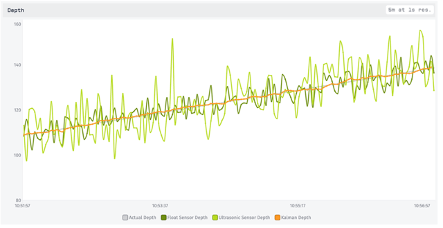
This really shows how much the Kalman value for depth is filtering out the noisy readings (green). We can also see how one of the sensors (light green) has more variation. Yet because the Kalman Filter adjusted for each sensor’s noise independently, the estimated value (orange) isn’t confused by this.
Kalman vs Simple Average
As discussed in part 1, we don’t always have to go to the lengths of implementing a complex Kalman Filter.
Here is the Kalman Filter time series graph together with our final approach from part 1, which used linear regression to create a predicted value that is combined with the new sensor readings using a weighted average:
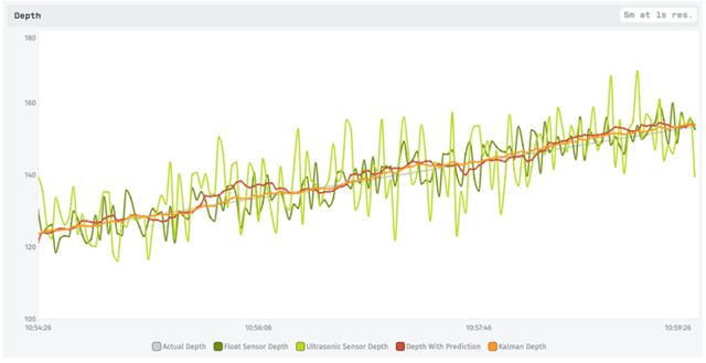
As you can see, the part 1 method in red does filter out some noise, but not quite as smoothly as the Kalman Filter estimate in orange.
To be fair, we could have continued taking steps to make the part 1 method more robust, such as considering variable sensor performance, adding in a process noise equivalent, and considering the velocity’s probability distribution in addition to the value’s probability distribution. However, as we take measures to try and get closer to the performance of a Kalman Filter, we are arguably just slowly building it up as one.
In our example the approaches are of similar mathematical complexity: one using more manual data transformations and calculations, one using linear algebra with matrix operations. While the Kalman Filter required implementing formulas that are less intuitive at first, it is easier to extend it once that foundation is in place. Adding additional sensors, dynamic sensor variances, the concept of acceleration (in addition to velocity), and even additional types of sensors are all relatively straightforward tasks.
Summary
Kalman Filters are extremely versatile. They are used in everything from missile tracking to self-driving cars. In our case, our final dashboard shows us exactly what we were aiming to accomplish. We have a less noisy estimate of the water depth, which still responds to true changes in the depth. We are also incorporating the readings of multiple sensors, each with its own accuracy, into this simple clean value. Finally, we have a reliable, human-friendly metric that gives us a new insight into our system—the rate of change—which is completely derived from the noisy estimates from the sensors.
To a large extent we were able to accomplish these without using a Kalman Filter in part 1. However, the Kalman Filter is more probabilistically thorough. Whereas our earlier attempts relied on various averages and the line of best-fit for past data, the Kalman Filter factored in highly-tunable uncertainties for each sensor and the current estimate of both depth and velocity. Using these, it gave us better noise reduction and a much more stable depth estimate.
As a final comparison, consider a case where the storm drain changed suddenly from filling to draining (+.1 cm/s to -.1 cm/s):
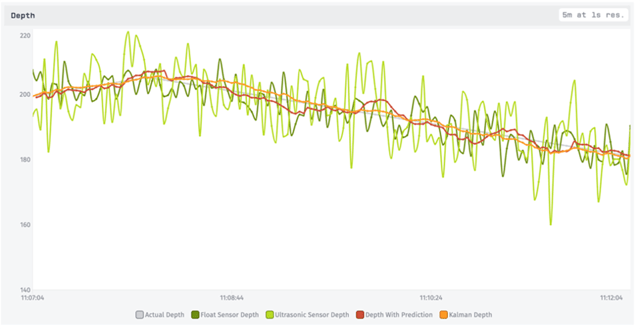
Both approaches stayed relatively close to the true values, but notice the red line from part 1 bouncing above and below the actual depth. It is having trouble converging to an estimate of the new rate of change, as seen more clearly in the velocity graph:
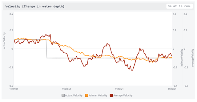
Over time with steady data it will converge more closely to the true value, but remember that it is simply using linear regression over the past 30 seconds, while the Kalman Filter is considering how much uncertainty it has in its own velocity estimate.
There are also variants and extensions of Kalman Filters that are commonly used. Perhaps most applicable here are variants that adjust the R (sensor noise) and Q (process noise) matrix dynamically based on the residuals, which are the differences between the new estimates and the sensor readings it observes. With this approach, we might create a filter that responds more quickly to changes. If our sensor readings are suddenly very different than what we’d expect, the filter would quickly lower its certainty about its ability to make predictions.
However, even the straightforward Kalman Filter we have created here resulted in an impressively accurate reduction of sensor noise.
This tutorial barely scratches the surface of Losant’s low-code platform. Please contact us to learn how Losant can help your organization deliver compelling IoT services for your customers.
|
Download to complete tutorial. (1.2 MB) |