
Sensor telemetry is at the heart of IoT. But while it can lead to amazing insights, it can also be noisy and inconsistent. There are two main sources of the problem. First, all sensors have hardware limitations and only measure to a certain degree of accuracy, with sequential readings having some amount of variance. (We call this variation in sensor readings, “sensor noise”.) Second, even if a sensor could measure with perfect accuracy and precision, the world itself that the sensor is measuring still presents variation; for instance, an IR distance sensor is affected by sunlight.
We can accept noise and inconsistency as a reality of IoT, but we can also take reasonable steps to reduce them. For instance, is there more accurate hardware available? Are there adjustable gain, sensitivity, positioning, or other calibrations to make on our sensors? Can we reduce environmental factors? Should we average out multiple readings over time? In many cases, these basic steps are enough to allow the data of interest to stand out.
But when more these basic steps have been pushed to their limits—or when they are impossible, impractical, or costly—we can use software techniques to filter out the noise and variation in readings. In this 2-part series, we will look at some approaches to reducing noise and gaining insight on the underlying data.
First, we will introduce a case study and attempt to solve it with the straightforward techniques of averages, running averages, and even weighted predictions using linear regression.
In the second part, we will add a more robust probabilistic technique to our toolkit known as Kalman Filtering. It will allow us to factor in sensor noise, combine data from multiple sensors, and use our knowledge about what we are monitoring to develop a dynamic model of our data.
Use Case: Monitoring the Water Level of a Storm Drain
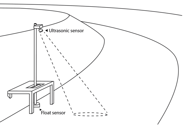
Let’s imagine we are monitoring a municipality’s storm drain system, and we want to know the current level of water at a certain point. For redundancy, we install two separate sensors: a float sensor that rests on top of the water, and an ultrasonic sensor mounted above the channel. The float sensor has an inherent accuracy of +/- 4 cm, but is heavily influenced by water churn, rising and falling with waves. The broad, cone shaped detection area of the ultrasonic sensor is not affected by churn, and its placement out of the water protects it. However, it is less accurate with greater distance to the water, ranging from +/- 1 cm at high water levels to +/- 10 cm at low water levels.
We also know that the water level tends to move in one direction or the other based on recent weather. Aside from small variations from surface turbulence, the water level will either be stable, rising, or falling, and won’t switch rapidly from one to another. So, in addition to filtering out some of the sensor noise to get a more accurate reading, we’d also like to get a sense of the water level’s current rate of change—something our sensors can’t directly measure—without getting misled by small variations in sensor readings. This could help us plan preemptive actions as the water approaches a critical depth.
Simulation Setup
Let’s talk about setting this up in Losant.
In our water level example, we have two sensors measuring the same thing. This could be set up as either two separate devices in Losant (one for each sensor) or as a single device reporting two depth attributes. We’ll choose the latter, as this would likely be data from out in the field, and there’s a good chance both sensors would report through a single gateway. So we add floatDepth and ultrasonicDepth as device attributes to a single device.
Finally, because this is a simulation, we will track the actual simulated depth of the water level and the actual rate of change. A production implementation would not have these values, and they are only ever shown in light gray on the dashboard charts.
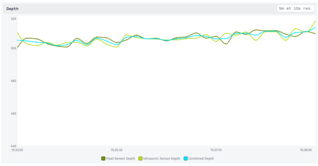
If our imaginary remote gateway supports MQTT, we can have it report device state directly to Losant. Then, without even having to set up a workflow, we can view the reported data using a Losant Dashboard with a Time Series Graph Block
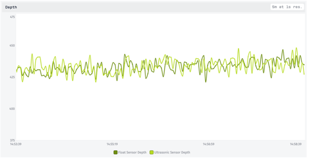
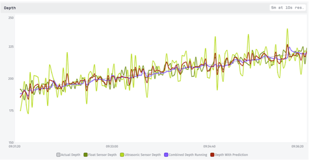
Here we see both sensors’ readings in green, with the natural variation and inaccuracy showing up clearly in the reported values. The light green line, representing the ultrasonic sensor, has more variance because the lower level of the water is not in its favor. More to the point, the water level is actually slowly rising here! It’s a gradual rate of only 2cm / minute, but because of all of the sensor noise, that’s very hard to tell visually. Our hope is to draw this feature out more clearly with the techniques below.
Reducing Noise with Aggregations and Simple Averages
Losant already provides us with some powerful aggregation features. The above chart was a 5 minute time series with a 1 second resolution and no aggregation. If we lower the resolution, we can choose to visualize the data using the mean, median, min, max, or several other aggregation methods.
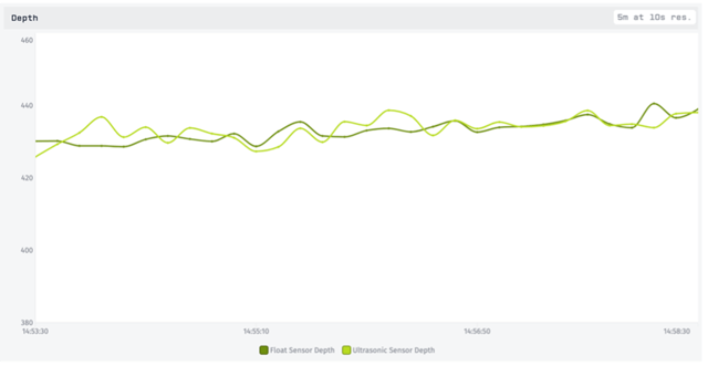
Using a 10 second resolution with the ‘mean’ aggregation method, we’ve already reduced a fair amount of the noise. However, this is a visual representation only and does not allow us to do much with the data. These are also both measuring the same depth, so a combined value would be even better. To accomplish this, we’ll set up a third device attribute called combinedDepth.
Combining Sensor Readings
The gateway is not reporting a combinedDepth for us, so we’ll need to listen to the reported state and calculate it ourselves. We can easily do this in a workflow with the Device: State Trigger:
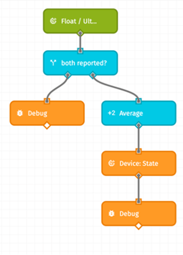 |
When floatDepth or ultrasonicDepth are reported, the workflow will trigger with that data. We are only interested if both sensors report, as we are calculating their average. Then we simply average them together and report the average to the new attribute. We are careful to select “Use the time of the current payload,” which will match the reporting time of the original state. |
|---|
Adding this third, computed attribute to our chart shows us that we have indeed combined our values together into a nice average:
We still have a 10 second mean aggregation, but now some of the individual sensor noise is balanced out by the other sensor. Still, when both sensors happen to report low or high together, we get artificial bumps in our average.
A Running Estimate
Since we are now tracking a computed value, we can go ahead and add a little more logic to it. One approach is to make this value more than an instantaneous average. It can instead look back at the previous values and combine them with the new readings for a running average. This should allow us to filter out some of the sensor noise by downplaying the variation in new values.
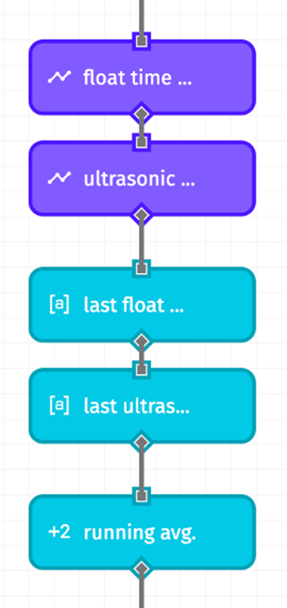 |
We add time series blocks to our workflow to query the past data for each of our sensor readings. One parameter here is how far back we want to look. For instance, we might choose to have a 30 second running average. We can let the Time Series Node provide us with the sum and count if we use one of the predefined resolutions and set the aggregation method to “mean”. We won’t use the mean value it gives us, because we want to first add in the new sensor readings. But the node helpfully provides both the “sum” and the “count” for us to add the new sensor readings to. |
|---|
Since the Time Series returns an array of points, we pull out the most recent one since that’s the one with values we are interested in.
Then we divide the result to get a running average:
{{working.lastFloatTimeSeriesPoint.sum}} +
{{working.lastUltrasonicTimeSeriesPoint.sum}} +
{{data.floatDepth}} + {{data.ultrasonicDepth}}
{{working.lastFloatTimeSeriesPoint.count}} +
{{working.lastUltrasonicTimeSeriesPoint.count}} + 2
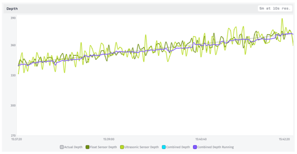
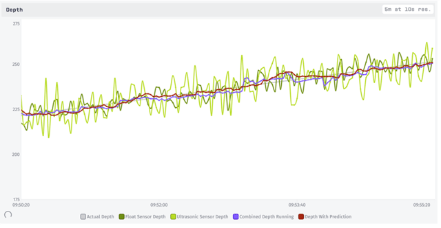
Adding this new value to our chart, we see a slightly less-variable line. Here it is pictured in purple:
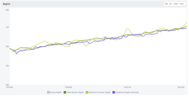
If we return our sensor readings (green) to their actual values we can see just how well the running average is performing. Overall this is giving us the best visual estimate so far.
You may notice, however, that it tends to be slightly low. That’s because our water level is rising, and incorporating past data will always drag a running average a bit into the past. We can address this with a different technique that involves estimating the rate of change—something we wanted to track anyways—and using it to make predictions.
Using Rate of Change to Predict Values
The rate that the water depth is changing is essentially a velocity, the formula for which is the change in value divided by the change in time:
| ν = | Δ x Δ t |
|---|
In our existing workflow, we can add a calculation of this by comparing past data across time. If we just use the last two data points to do this, though, the velocity will rapidly fluctuate due to the sensor noise. Instead we’d like to get an average recent velocity. There’s more than one way to do this, but a sensible method is using simple linear regression. We have a scatterplot of values and times, so finding the best fitting line through these points will yield the velocity in the form of the line’s slope.
To use linear regression with a time series, time is our independent variable (x) and the value is our dependent variable (y). We replace the timestamps with an epoch time equivalent so that they are plottable integers, but to keep the numbers lower, we subtract off 1,650,000,000. Now our epoch value represents “seconds since April 15, 2022” instead of “seconds since January 1, 1970”.
For the linear regression calculation itself, it’s more straightforward to jump into a Function Node.
With the slope and intercept of the best-fitting line, we can now extend the line of best fit to the current time, and we’ll be looking at a loose but reasonable prediction of the value. Then we can average this prediction in with sensor readings to create an estimate. This approach should allow good estimates even when the depth is rising or falling:
The prediction depth initially performs worse than the running average. Why? Because the running average gives equal weight to each of the past data points and the new sensor readings, while the prediction depth combines all the past data into a single point. Instead of new sensor readings making up 3% (2 out of 62 data points) of the new value with a running average, they make up 66% (2 out of 3 data points) of the new value with the prediction.
However, we can easily adjust the weight of our prediction. In fact, giving it the same ratio as the running average results in a similar value, but one that is aware of rate of change!
That’s not bad, and we could play around with this weight more to find a value that is smooth but still responsive to new data.
Visualizing the Rate of Change
Since we are already calculating the line that best fits the recent data, we can use its slope as an estimate of the water level’s rate of change, or velocity. We add another attribute to our device, velocityEstimate, and save the value as state at the same time as our prediction.
We’ll show this estimate in a few different ways on our final dashboard: as a simple value using a Gauge, as a value over time with a Time Series Graph, and as a human friendly summary using an Indicator:
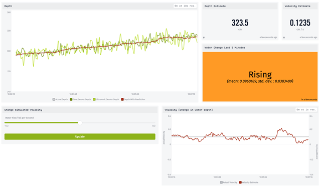
At the time of the screenshot, the simulated velocity was set to +0.1 cm/s. We can see in the velocity graph (bottom-right) that our estimated velocity is hovering fairly close to the true value. We’ve also added an indicator block showing a human-friendly summary of the velocity: whether it is rising, falling, or stable:
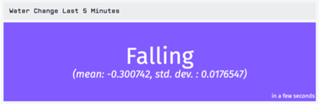
This block uses the estimated rate of change. However, that specific value is a little too variable, because it’s constantly adjusting our estimated depth up and down to track the water level. We need to average this out a little over time, and consider how much it’s deviating.
In the Indicator Block, we consider both the mean of the estimated velocity as well as its standard deviation over a period of time (5 minutes). If the standard deviation is larger than the velocity’s distance from 0 (say, a mean of 0.1 with a standard deviation of 1) we can’t be very confident about whether the level is rising or falling. So if we have a high standard deviation, we choose to report this as “Fluctuating” rather than give a bad estimate.
Summary
We’ve taken 2 sensors giving quite noisy data and used various techniques to filter it out and derive actionable insights. First, we used the dashboard blocks’ built-in aggregation to get a smoother visualization of the data. Next, we created a combined depth reading that factored in both sensors. Then we brought in past data to smooth out the combined value as a running average. Finally, we used linear regression to estimate the depth’s rate of change and create a predicted value, which we were able to weigh with the actual observations.
All of these techniques allowed us to view our data with less noise. The linear regression prediction, though, also gave us a deduced value of the water depth’s velocity. With this we were able to add a simple, actionable indicator to our dashboard.
We could combine some of these techniques, or continue to refine them. For instance, since we know the ultrasonic sensor’s accuracy changes with the water depth, we could weigh its value accordingly based on the depth. However, we’ll instead shift gears in the second part of this series to look at Kalman Filters. It will incorporate many of the same principles we’ve used here, but in a more cohesive way that considers various probabilities from the very beginning. Our work in this first part will serve as an excellent baseline against which we can compare our Kalman Filters performance, which we will explore in part 2.
This tutorial barely scratches the surface of Losant’s low-code platform. Please contact us to learn how Losant can help your organization deliver compelling IoT services for your customers.
|
Download to complete tutorial. (1.2 MB) |